Learning edge direction in a Bayesian network model
Taken from coursework for ECE 7751: Graphical Models in Machine Learning, taught by Faramarz Fekri at Georgia Tech, Spring 2023
Our interest here is to discuss a method to learn the direction of an edge in a belief network. Consider a distribution $$ P(x,y | \theta,M_{y\to x}) = P(x|y,\theta_{x|y})P(y|\theta_y) $$
where $\theta$ are the parameters of the conditional probability tables. For a prior $p(\theta)=p(\theta_{x|y})p(\theta_y)$ and i.i.d. data $\mathcal{D}= \lbrace x^n,y^n,n=1,…,N\rbrace$, the likelihood of the data is
$$ p(\mathcal{D}|M_{y\to x}) = \int_\theta p(\theta_{x|y})p({\theta_y}) \prod_n p(x^n|y^n,\theta_{x|y})p(y^n|\theta_y) $$
For binary variables $x\in \lbrace 0,1\rbrace,y\in\lbrace 0,1\rbrace$,
$$ p(y=1|\theta_y) = \theta_y, \qquad p(x=1|y,\theta_{x|y})=\theta_{1|y} $$
and Beta distribution priors
$$ p(\theta_y) = B(\theta_y|\alpha,\beta),\qquad p(\theta_{1|y}) = B(\theta_{1|y}|\alpha_{1|y},\beta_{1|y}), \qquad p(\theta_{1|1}\theta_{1|0} = p(\theta_{1|1})p(\theta_{1|0}). $$
Expanding the formula for $P(\mathcal{D}|M_{y\to x})$
Find a formula to estimate
$$ P(\mathcal{D}|M_{y\to x}) $$
in terms of parameters of Beta priors and the actual counts in training data.
Figure 1: Two alternative structures for a belief network
Solution
$$ \begin{aligned} P(\mathcal{D}|M_{y\to x}) &= \int_\theta p(\theta_y)p(\theta_{x|y})\prod_n p(y^n|\theta_y)p(x^n|y^n,\theta_{x|y})d\theta \\ &= \int_\theta \left( \begin{aligned} &B(\alpha_{y},\beta_{y})\theta_{y}^{\alpha-1}\left(1-\theta_{y}\right)^{\beta-1} B(\alpha_{x|1},\beta_{x|1})\theta_{x|1}^{\alpha_{x|1}-1}\left(1-\theta_{x|1}\right)^{\beta_{x|1}-1} B(\alpha_{x|0},\beta_{x|0})\theta_{x|0}^{\alpha_{x|0}-1}\left(1-\theta_{x|0}\right)^{\beta_{x|0}-1} \\ &*\theta_{y}^{N_{y=1}}\left(1-\theta_{y}\right)^{N_{y=0}} \theta_{1|1}^{N_{1|y=1}}\left(1-\theta_{1|1}\right)^{N_{0|y=1}} \theta_{1|0}^{N_{1|y=0}}\left(1-\theta_{1|0}\right)^{N_{0|y=0}} \\ \end{aligned} \right) d\theta \\ &= \int_\theta \left( \begin{aligned} &B(\alpha_{y},\beta_{y})\theta_{y}^{N_{y=1}+\alpha-1}\left(1-\theta_{y}\right)^{N_{y=0}+\beta-1} \\ &B(\alpha_{x|1},\beta_{x|1})\theta_{x|1}^{N_{1|y=1}+\alpha_{x|1}-1}\left(1-\theta_{x|1}\right)^{N_{0|y=1}+\beta_{x|1}-1} \\ &B(\alpha_{x|0},\beta_{x|0})\theta_{x|0}^{N_{1|y=0}+\alpha_{x|0}-1}\left(1-\theta_{x|0}\right)^{N_{0|y=0}+\beta_{x|0}-1} \\ \end{aligned} \right) d\theta \\ &= \left(\begin{aligned} &\int_{\theta_y}B(\alpha_{y},\beta_{y})\theta_{y}^{N_{y=1}+\alpha-1}\left(1-\theta_{y}\right)^{N_{y=0}+\beta-1}d\theta_y \\ &*\int_{\theta_{x|1}}B(\alpha_{x|1},\beta_{x|1})\theta_{x|1}^{N_{1|y=1}+\alpha_{x|1}-1}\left(1-\theta_{x|1}\right)^{N_{0|y=1}+\beta_{x|1}-1}d{\theta_{x|1}} \\ &*\int_{\theta_{x|0}}B(\alpha_{x|0},\beta_{x|0})\theta_{x|0}^{N_{1|y=0}+\alpha_{x|0}-1}\left(1-\theta_{x|0}\right)^{N_{0|y=0}+\beta_{x|0}-1}d{\theta_{x|0}} \\ \end{aligned}\right) \\ &= \textcolor{Green}{\fbox{$B(\alpha+N_{y=1},\beta+N_{y=0})B(\alpha_{x|1}+N_{1|y=1},\beta_{x|1}+N_{0|y=1})B(\alpha_{x|0}+N_{1|y=0},\beta_{x|0}+N_{0|y=0})$}} \\ \end{aligned} $$Expanding the formula for $P(\mathcal{D}|M_{x\to y})$
Now derive a similar expression as in part 1 for the model with the edge direction reversed,
$$ P(\mathcal{D}|M_{x\to y}) $$
assuming the same values (as in part 1, except that the role of $x$ and $y$ are switched) for all hyperparameters of this reverse model.
Solution
Same as above, but switching $x$ and $y$:
$$ \begin{aligned} P(\mathcal{D}|M_{x\to y}) &= \textcolor{Green}{\fbox{$B(\alpha+N_{x=1},\beta+N_{x=0})B(\alpha_{y|1}+N_{1|x=1},\beta_{y|1}+N_{0|x=1})B(\alpha_{y|0}+N_{1|x=0},\beta_{y|0}+N_{0|x=0})$}} \\ \end{aligned} $$
Deriving the Bayes factor
Using the above, derive a simple expression for the Bayes’ factor, which computes the ratio of probability you found in part 1 to probability in part 2:
$$ \frac{P(\mathcal{D}|M_{y\to x})}{P(\mathcal{D}|M_{x\to y})} $$
Solution
$$ \begin{aligned} &\frac{P(\mathcal{D}|M_{y\to x})}{P(\mathcal{D}|M_{x\to y})} = \\ &\quad\textcolor{Green}{\fbox{$\frac{ B(\alpha+N_{y=1},\beta+N_{y=0})B(\alpha_{x|1}+N_{1|y=1},\beta_{x|1}+N_{0|y=1})B(\alpha_{x|0}+N_{1|y=0},\beta_{x|0}+N_{0|y=0}) }{ B(\alpha+N_{x=1},\beta+N_{x=0})B(\alpha_{y|1}+N_{1|x=1},\beta_{y|1}+N_{0|x=1})B(\alpha_{y|0}+N_{1|x=0},\beta_{y|0}+N_{0|x=0}) }$}} \end{aligned} $$
Leveraging priors to choose the more deterministic model
By choosing appropriate hyperparameters (i.e., beta priors), give a numerical example that illustrates how to encode the heuristic that if the table $p(x|y)p(y)$ is ‘more deterministic’ than $p(y|x)p(x)$, then we should prefer the model $M_{y\to x}$. (Note that when we say is ‘more deterministic’ that implies that given $y$, the outcome of $x$ is quite certain (e.g., to be zero).)
Compute the Bayes factor for the situation
| y=0 | y=1 | |
|---|---|---|
| x=0 | 10 | 10 |
| x=1 | 0 | 0 |
And also compare the resulting Bayes factor in the above situation but use a uniform prior for all priors instead.
Solution
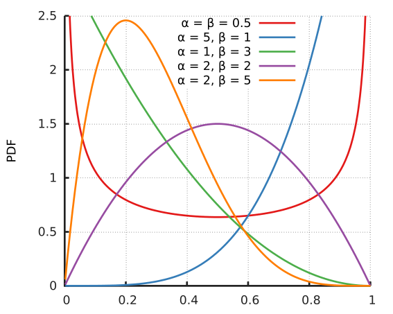
We use the same hyperparameters for both models (e.g., the same $\alpha$ and $\beta$ for both $p(y)$ and $p(x)$), for a fair, uninformed comparison. Using $\alpha_{a|b}=\beta_{a|b}<1/2$ corresponds to favoring $\theta_{a|b}$ close to 0 or 1, that is, more deterministic models. $\alpha=\beta=\frac{1}{2}$ is what is called the Jeffreys prior, and is considered the truly ‘uninformed’ prior, favoring neither deterministic or entropic distributions.
This image from Wikipedia illustrates the effect of different priors on the beta distribution:
import numpy as np
from scipy.special import beta as B, gamma as G

def bayes_factor(xy00, xy01, xy10, xy11, alpha1, beta1, alpha11, beta01, alpha10, beta00):
    N = xy00 + xy01 + xy10 + xy11
    Ny1 = xy01 + xy11
    Ny0 = xy00 + xy10
    Nx1 = xy10 + xy11
    Nx0 = xy00 + xy01
    res = B(alpha1 + Ny1, beta1 + Ny0) / B(alpha1 + Nx1, beta1 + Nx0) \
        * B(alpha11 + xy11, beta01 + xy01) / B(alpha11 + xy11, beta01 + xy10) \
        * B(alpha10 + xy10, beta00 + xy00) / B(alpha10 + xy01, beta00 + xy00)
    return res

def bayes_test(alphabeta, alphabeta_cond):
    res = bayes_factor(10, 10, 0, 0, alphabeta, alphabeta, alphabeta_cond, alphabeta_cond, alphabeta_cond, alphabeta_cond)
    if np.isclose(res, 1, rtol=1e-3):
      print(f'Bayes factor = {res}, neither model preferred')
    elif res > 1:
      print(f'Bayes factor = {res}, My->x preferred')
    elif res < 1:
      print(f'Bayes factor = {res}, Mx->y preferred')

bayes_test(.5, .2)
Bayes factor = 1.4689932412843798, My->x preferred
This is as expected.
We get a stronger preference for $M_{y\to x}$ if we use a uniform rather than a Jeffreys prior for $\alpha,\beta$, since the marginal distribution of $y$ is more entropic (uniform) than that of $x$ (there are no samples with $x=1$). This is what we should use to make our decision, since it means we don’t care about whether $\theta$ produces stochastic or deterministic marginal $x$ and $y$.
bayes_test(1, .2)
Bayes factor = 5.932237498634842, My->x preferred
We can confirm that the Jeffreys prior does indeed prefer neither model:
bayes_test(1, .5)
Bayes factor = 1.0, neither model preferred
If we use the Jeffreys prior for both parent and conditional parameters, $M_{x\to y}$ is preferred since it better balances stochastic and deterministic distributions.
bayes_test(.5, .5)
Bayes factor = 0.24762886543609094, Mx->y preferred
Finally, using uniform priors as requested, $M_{x\to y}$ is preferred, as we would expect:
bayes_test(1, 1)
Bayes factor = 0.17355371900826447, Mx->y preferred
Kyle Johnsen
PhD Candidate, Biomedical Engineering
My research interests include applying principles from the brain to improve machine learning.