Mean field variational inference
Taken from coursework for ECE 7751: Graphical Models in Machine Learning, taught by Faramarz Fekri at Georgia Tech, Spring 2023
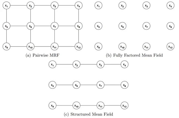 A pairwise Markov Random Field and the structure of two mean field approximations
In this problem, you will investigate mean field approximate inference algorithms (Koller & Friedman1 11.5). Consider the Markov network in the above figure. Define edge potentials $\phi_{ij}(x_i,x_j)$ for all edges $(x_i , x_j)$ in the graph. We can write
$$ P\left(x_1, \ldots, x_{12}\right)=\frac{1}{Z} \prod_{(i, j) \in E} \phi_{i j}\left(x_i, x_j\right) $$
Fully factored mean field
Assume a fully factored mean field approximation $Q$ (b in figure), parameterized by node potentials $Q_i$.
In both of the cases below, please expand out any expectations in the formulas (your answer should be in terms of $Q_i$ and $\phi_{ij}$).
Write down the update formulas for $Q_1(X_1)$ and $Q_6(X_6)$.
Solution
$Q_1(X_1)$
Using the update formula for a fully factored mean field, where $D_j$ represents clique $j$,
$$ \begin{aligned} Q_i(X_i) &= \frac{1}{Z_i} \exp\left(\sum_{D_j: X \in D_j} \mathbb{E}_{Q_{-i}} \ln \phi(D_j)\right) \\ Q_1(X_1) &= \frac{1}{Z_1} \exp\left(\mathbb{E}_{Q_{2}} \ln \phi(X_1,X_2) + \mathbb{E}_{Q_{5}} \ln \phi(X_1,X_5)\right) \\ &= \color{Green} \frac{1}{Z_1} \exp\left(\sum_{X_2} Q_2(X_2) \ln\phi(X_1,X_2) + \sum_{X_5} Q_5(X_5) \ln\phi(X_1,X_5)\right) \\ \end{aligned} \newcommand{\EE}{\mathbb{E}} \newcommand{\ind}{\mathbb{1}} \newcommand{\answertext}[1]{\textcolor{Green}{\fbox{#1}}} \newcommand{\answer}[1]{\answertext{$#1$}} \newcommand{\argmax}[1]{\underset{#1}{\operatorname{argmax}}} \newcommand{\argmin}[1]{\underset{#1}{\operatorname{argmin}}} \newcommand{\comment}[1]{\textcolor{gray}{\textrm{#1}}} \newcommand{\vec}[1]{\mathbf{#1}} \newcommand{\inv}[1]{\frac{1}{#1}} \newcommand{\abs}[1]{\lvert{#1}\rvert} \newcommand{\norm}[1]{\lVert{#1}\rVert} \newcommand{\lr}[1]{\left(#1\right)} \newcommand{\lrb}[1]{\left[#1\right]} \newcommand{\lrbr}[1]{\lbrace#1\rbrace} \newcommand{\Bx}[0]{\mathbf{x}} $$$Q_6(X_6)$
The derivation is similar to the previous part:
$$ \begin{multline} Q_6(X_6) = \color{Green} \frac{1}{Z_1} \exp\Biggl( \sum_{X_2} Q_2(X_2)\ln \phi(X_2,X_6) + \sum_{X_5} Q_5(X_5) \ln\phi(X_5,X_6) \\ \color{Green} + \sum_{X_7} Q_7(X_7)\ln \phi(X_6,X_7) + \sum_{X_{10}} Q_{10}(X_{10})\ln \phi(X_6,X_{10}) \Biggr) \end{multline} $$Structured mean field
Now we consider a structured mean field approximation $Q$ (c in figure), parameterized by edge potentials $\psi_{ij}(x_i,x_j)$ for each edge $(x_i , x_j)$.
$\psi_{12}(x_1,x_2)$
Write down the update formula for $\psi_{12}(x_1,x_2)$ up to a proportionality constant. This time, you can write it in terms of expected values, but do not include unnecessary terms.
Solution
We start with equation (11.62) from Koller & Friedman1: $$ \psi_j\left(D_j\right) \propto \exp \left\{\sum_{\phi \in A_j} \mathbb{E}_{\mathcal{X} \sim Q}\left[\ln \phi \mid D_j\right]-\sum_{\psi_k \in B_j} \mathbb{E}_{\mathcal{X} \sim Q}\left[\ln \psi_k \mid D_j\right]\right\}, $$
where
$$ A_j=\left\{\phi \in \Phi: Q \not \models\left(\mathbf{U}_\phi \perp \mathbf{D}_j\right)\right\} $$ $$ B_j=\left\{\psi_k: Q \not \models\left(\mathbf{D}_k \perp \mathbf{D}_j\right)\right\}-\left\{\mathbf{D}_j\right\}. $$$Q \not\models$ means that the statement is not true in $Q$ and $\mathbf{U}_\phi$ refers to all variables involved in the factor $\phi$. These $A_j$ and $B_j$ sets essentially include factors that are not independent from the clique $D_j$ in our approximate distribution $Q$.
Thus, we have
$$ \newcommand{\EE}{\mathbb{E}} \begin{multline} \psi_{12}(x_1,x_2) \propto \\ \color{Green} \exp \left( \begin{aligned} &\mathbb{E}_Q[\ln\phi_{12}(x_1,x_2)|x_1,x_2] + \mathbb{E}_Q[\ln\phi_{23}(x_2,x_3)|x_1,x_2] + \mathbb{E}_Q[\ln\phi_{34}(x_3,x_4)|x_1,x_2]) \\ &+ \mathbb{E}_Q[\ln\phi_{15}(x_1,x_5)|x_1,x_2] + \mathbb{E}_Q[\ln\phi_{26}(x_2,x_6)|x_1,x_2] + \mathbb{E}_Q[\ln\phi_{37}(x_3,x_7)|x_1,x_2]) + \mathbb{E}_Q[\ln\phi_{48}(x_4,x_8)|x_1,x_2]) \\ &- \mathbb{E}_Q[\ln\psi_{23}(x_2,x_3)|x_1,x_2] - \mathbb{E}_Q[\ln\psi_{34}(x_3,x_4)|x_1,x_2]) \\ \end{aligned} \right) \end{multline} $$$\mathbb{E}_Q[\ln\phi_{26}(X_2,X_6)|x_1,x_2]$
Write out the formula for $\mathbb{E}Q[\ln\phi{26}(X_2,X_6)|x_1,x_2]$. Make sure to show how you would calculate the distribution that this expectation is over.
Solution
We only need to take the expectation over the variables in the function:
$$ \EE_{Q(X_1,\ldots,X_N)} f(X_1) = \EE_{Q(X_1)}f(X_1) $$
Also, we need not take the expectation over a variable being conditioned on: $$ \EE_{Q(X_1, X_2|x_1)}[f(X_1,X_2)] = \EE_{Q(X_2|x_1)}[f(x_1, X_2)] $$
Hence, $$ \begin{aligned} &\EE_{Q(X_1,\ldots,X_n)}[\ln\phi_{26}(X_2,X_6)|x_1,x_2] \\ &= \EE_{Q(X_1,\ldots,X_n|x_1,x_2)}\ln\phi_{26}(X_2,X_6) \\ &= \EE_{Q(X_6|x_1,x_2)}\ln\phi_{26}(X_2,X_6). \\ &= \EE_{Q(X_6|x_1,x_2)}\ln\phi_{26}(x_2,X_6). \\ &= \EE_{Q(X_6)}\ln\phi_{26}(x_2,X_6) &\color{Gray}\textsf{since $X_6 \perp X_1,X_2$ in $Q$} \\ \end{aligned} $$ $$ \begin{aligned} Q(X_6) &= \sum_{\mathcal{X}\backslash\lrbr{X_6}} Q(X_1,\ldots,X_n) \\ &= \sum_{x_5,x_7,x_8} Q(X_5,X_6,X_7,X_8) \\ &= \inv{Z_{C_2}} \sum_{x_5,x_7,x_8} \psi(X_5,X_6)\psi(X_6,X_7)\psi(X_7,X_8) \\ \end{aligned} $$ $$ \color{Green} \EE_Q[\ln\phi_{26}(X_2,X_6)|x_1,x_2] = \inv{Z_{C_2}}\sum_{x_5,x_6,x_7,x_8} \ln\phi(x_2,x_6)\psi(x_5,x_6)\psi(x_6,x_7)\psi(x_7,x_8)\\ $$
$\EE_Q[\ln\phi_{15}(X_1,X_5)|x_1,x_2]$
Write out the formula for $\EE_Q[\ln\phi_{15}(X_1,X_5)|x_1,x_2]$. Again, show how you would evaluate distribution $Q$.
Solution
We follow the same steps and arrive at a very similar answer:
$$ \color{Green} \EE_Q[\ln\phi_{15}(X_1,X_5)|x_1,x_2] = \inv{Z_{C_2}} \sum_{x_5,x_6,x_7,x_8} \ln\phi(x_1,x_5)\psi(x_5,x_6)\psi(x_6,x_7)\psi(x_7,x_8)\\ $$Kyle Johnsen
PhD Candidate, Biomedical Engineering
My research interests include applying principles from the brain to improve machine learning.